JPEG:-
- "Joint Photographic Expert Group" -- an international standard in 1992.
- Works with color and grey scale images, Many applications e.g., satellite, medical, ...
-
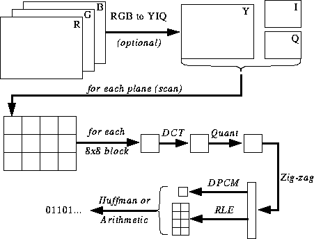
JPEG Encoding
- Decoding - Reverse the order for encoding
- DCT (Discrete Cosine Transformation)
- Quantization
- Zigzag Scan
- DPCM on DC component
- RLE on AC Components
- Entropy Coding
Quantization
Why do we need to quantise:- To throw out bits
- Example: 101101 = 45 (6 bits).
Truncate to 4 bits: 1011 = 11.
Truncate to 3 bits: 101 = 5.
- Quantization error is the main source of the Lossy Compression
Uniform quantization
- Divide by constant N and round result (N = 4 or 8 in examples above).
- Non powers-of-two gives fine control (e.g., N = 6 loses 2.5 bits)
Quantization Tables
- In JPEG, each F[u,v] is divided by a constant q(u,v).
- Table of q(u,v) is called quantization table.
----------------------------------
16  11  10  16  24   40   51   61
12  12  14  19  26   58   60   55
14  13  16  24  40   57   69   56
14  17  22  29  51   87   80   62
18  22  37  56  68   109  103  77
24  35  55  64  81   104  113  92
49  64  78  87  103  121  120  101
72  92  95  98  112  100  103  99
----------------------------------
- Eye is most sensitive to low frequencies (upper left corner), less sensitive to high frequencies (lower right corner)
- Standard defines 2 default quantization tables, one for luminance (above), one for chrominance.
- Q: How would changing the numbers affect the picture (e.g., if I doubled them all)?
Quality factor in most
implementations is the scaling factor for default quantization tables.
- Custom quantization tables can be put in image/scan header.
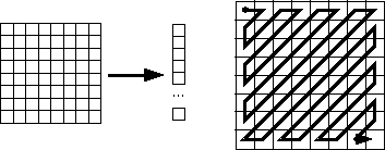
Zig-zag Scan
What is the purpose of the Zig-zag Scan:- to group low frequency coefficients in top of vector.
- Maps 8 x 8 to a 1 x 64 vector
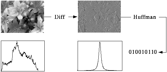
Differential Pulse Code Modulation (DPCM) on DC component
Here we see that besides DCT another encoding method is employed: DPCM on the DC component at least. Why is this strategy adopted: - DC component is large and varied, but often close to previous value (like lossless JPEG).
- Encode the difference from previous 8x8 blocks - DPCM
Run Length Encode (RLE) on AC components
Yet another simple compression technique is applied to the AC component:- 1x64 vector has lots of zeros in it
- Encode as (skip, value) pairs, where skip is the number of zeros and value is the next non-zero component.
- Send (0,0) as end-of-block sentinel value.
Entropy Coding
DC and AC components finally need to be represented by a smaller number of bits:- Categorize DC
values into SSS (number of bits needed to represent) and actual bits.
-------------------- Value SSS 0 0 -1,1 1 -3,-2,2,3 2 -7..-4,4..7 3 -------------------- - Example: if DC value is 4, 3 bits are needed.
Send off SSS as Huffman symbol, followed by actual 3 bits.
- For AC components (skip, value), encode the composite symbol (skip,SSS) using the Huffman coding.
- Huffman Tables can be custom (sent in header) or default.
Summary of the JPEG bitstream
Above JPEG components have described how compression is achieved at several stages. Let us conclude by summarizing the overall compression process:- A "Frame" is a picture, a "scan" is a pass through the pixels (e.g., the red component), a "segment" is a group of blocks, a "block" is an 8x8 group of pixels.
- Frame header: sample precision (width, height) of image number of components unique ID (for each component) horizontal/vertical sampling factors (for each component) quantization table to use (for each component)
- Scan header Number of components in scan component ID (for each component) Huffman table for each component (for each component)
- Misc. (can occur between headers) Quantization tables Huffman Tables Arithmetic Coding Tables Comments Application Data
Practical JPEG Compression
JPEG compression algorithms may fall in to one of several categories depending on how the compression is actually performed:- Baseline/Sequential - the one that we described in detail
- Lossless
- Progressive
- Hierarchical
- "Motion JPEG" - Baseline JPEG applied to each image in a video.
- 1.
- Lossless Mode
- A special case of the JPEG where indeed there is no loss
- Take difference from previous pixels (not blocks as in the
Baseline mode) as a "predictor".
Predictor uses linear combination of previously encoded neighbors.
It can be one of seven different predictor based on pixels neighbors
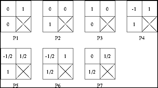
- Since it uses only previously encoded neighbors, first row always uses P2, first column always uses P1.
- Effect of Predictor (test with 20 images)
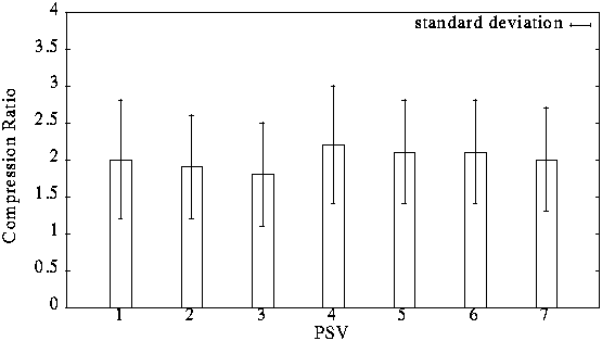
Note: "2D" predictors (4-7) always do better than "1D" predictors.
----------------------------------------------------------------- Compression Program Compression Ratio Lena football F-18 flowers ----------------------------------------------------------------- lossless JPEG 1.45 1.54 2.29 1.26 optimal lossless JPEG 1.49 1.67 2.71 1.33 compress (LZW) 0.86 1.24 2.21 0.87 gzip (Lempel-Ziv) 1.08 1.36 3.10 1.05 gzip -9 (optimal Lempel-Ziv) 1.08 1.36 3.13 1.05 pack (Huffman coding) 1.02 1.12 1.19 1.00 ----------------------------------------------------------------- - A special case of the JPEG where indeed there is no loss
- 2.
- Progressive Mode
- Goal: display low quality image and successively improve.
- Two ways to successively improve image:
- (a)
- Spectral selection: Send DC component, then first few AC, some more AC, etc.
- (b)
- Successive approximation: send DCT coefficients MSB (most significant bit) to LSB (least significant bit).
- 3.
- Hierarchical Mode
A Three-level Hierarchical JPEG Encoder
(From V. Bhaskaran and K. Konstantinides, "Image and Video Compression Standards: Algorithms and Architectures", Kluwer Academic Publishers, 1995.)
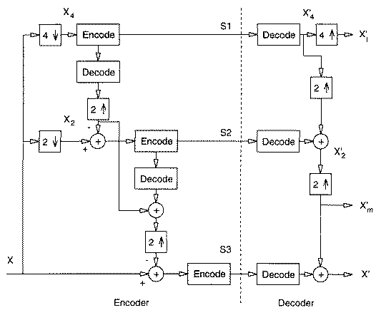
- Down-sample by factors of 2 in each direction.
Example: map 640x480 to 320x240
- Code smaller image using another method (Progressive, Baseline, or Lossless).
- Decode and up-sample encoded image
- Encode difference between the up-sampled and the original using Progressive, Baseline, or Lossless.
- Can be repeated multiple times.
- Good for viewing high resolution image on low resolution display.
- Down-sample by factors of 2 in each direction.
Example: map 640x480 to 320x240
- 4
- JPEG-2
- Big change was to use adaptive quantization
MPEG Compression
The acronym MPEG stands for Moving Picture Expert Group, which worked to generate the specifications under ISO, the International Organization for Standardization and IEC, the International Electrotechnical Commission. What is commonly referred to as "MPEG video" actually consists at the present time of two finalized standards, MPEG-11 and MPEG-22, with a third standard, MPEG-4, was finalized in 1998 for Very Low Bitrate Audio-Visual Coding. The MPEG-1 and MPEG-2 standards are similar in basic concepts. They both are based on motion compensated block-based transform coding techniques, while MPEG-4 deviates from these more traditional approaches in its usage of software image construct descriptors, for target bit-rates in the very low range, < 64Kb/sec. Because MPEG-1 and MPEG-2 are finalized standards and are both presently being utilized in a large number of applications, this paper concentrates on compression techniques relating only to these two standards. Note that there is no reference to MPEG-3. This is because it was originally anticipated that this standard would refer to HDTV applications, but it was found that minor extensions to the MPEG-2 standard would suffice for this higher bit-rate, higher resolution application, so work on a separate MPEG-3 standard was abandoned.MPEG video compression technique

That means a
Java program must buffer at least three frames: One for
forward prediction and one for backward prediction. The third buffer contains the frame coming into being.
As the figure shows the frame for backward prediction follows the predicted frame. That would
require to suspend the decoding of B-frames till the next P- or B- frame appears. But fortunately
the display order is not the coding order. The frames appear on MPEG data stream in such an order that the referred
frames precede the referring frames.The discrete cosine transform(DCT):
| As mentioned above the 8x8 block values are coded by means of the discrete cosine transform. To explain this regard the figure to the right. This shall be an enlargement of an 8x8 area of a black-white frame. |  |
| The normal way is to determine the brightness of each of the 64 pixels and to scale them to some limits, say from 0 to 255*, whereby "0" means "black" and "255" means "white". We can also represent the values in form of an 8x8 bar diagram. Normally the values are processed line by line. That requires 64 byte of storage. |


f(x,y) is the brightness of the pixel at position [x,y]. The result is F
an 8x8 array, too:
|
But as you can see: almost all values are equal to zero. Because the non-zero values are concentrated
at the upper left corner the matrix is transfered to the receiver in zigzag scan order. That would result in: 700 90 90 -89 0 100 0 0 0 .... 0 Of course, the zeros are not transferred. An End-Of-Block sign is coded instead. |
 |
 Where
Where F(u,v) is the transform matrix value at position [u,v]. The results are
exactly the original pixel values. Therefore the MPEG compression could be regarded as loss-less. But that isn't true,
because the transformed values are quantized. That means they are (integer) divided by a certain value greater or
equal 8 because the DCT supplies values up to 2047. To reduce them under the byte length at least the
quantization value 8 is applied. The decoder multiplies the result by the same value. Of course the
result differs from the original value. But again because of some properties of the human eye the error isn't
visible. In MPEG there is a quantization matrix which defines a different quantization value for every
transform value depending on its position.MPEG Video Layers
MPEG video is broken up into a hierarchy of layers to help with error handling, random search and editing, and synchronization, for example with an audio bitstream. From the top level, the first layer is known as the video sequence layer, and is any self-contained bitstream, for example a coded movie or advertisement. The second layer down is the group of pictures, which is composed of 1 or more groups of intra (I) frames and/or non-intra (P and/or B) pictures that will be defined later. Of course the third layer down is the picture layer itself, and the next layer beneath it is called the slice layer. Each slice is a contiguous sequence of raster ordered macroblocks, most often on a row basis in typical video applications, but not limited to this by the specification. Each slice consists of macroblocks, which are 16x16 arrays of luminance pixels, or picture data elements, with 2 8x8 arrays of associated chrominance pixels. The macroblocks can be further divided into distinct 8x8 blocks, for further processing such as transform coding. Each of these layers has its own unique 32 bit start code defined in the syntax to consist of 23 zero bits followed by a one, then followed by 8 bits for the actual start code. These start codes may have as many zero bits as desired preceding them.B-Frames
The MPEG encoder also has the option of using forward/backward interpolated prediction. These frames are commonly referred to as bi-directional interpolated prediction frames, or B frames for short. As an example of the usage of I, P, and B frames, consider a group of pictures that lasts for 6 frames, and is given as I,B,P,B,P,B,I,B,P,B,P,B,� As in the previous I and P only example, I frames are coded spatially only and the P frames are forward predicted based on previous I and P frames. The B frames however, are coded based on a forward prediction from a previous I or P frame, as well as a backward prediction from a succeeding I or P frame. As such, the example sequence is processed by the encoder such that the first B frame is predicted from the first I frame and first P frame, the second B frame is predicted from the second and third P frames, and the third B frame is predicted from the third P frame and the first I frame of the next group of pictures. From this example, it can be seen that backward prediction requires that the future frames that are to be used for backward prediction be encoded and transmitted first, out of order. This process is summarized in Figure. There is no defined limit to the number of consecutive B frames that may be used in a group of pictures, and of course the optimal number is application dependent. Most broadcast quality applications however, have tended to use 2 consecutive B frames (I,B,B,P,B,B,P,�) as the ideal trade-off between compression efficiency and video quality.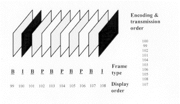
B-Frame Encoding The main advantage of the usage of B frames is coding efficiency. In most cases, B frames will result in less bits being coded overall. Quality can also be improved in the case of moving objects that reveal hidden areas within a video sequence. Backward prediction in this case allows the encoder to make more intelligent decisions on how to encode the video within these areas. Also, since B frames are not used to predict future frames, errors generated will not be propagated further within the sequence.
One disadvantage is that the frame reconstruction memory buffers within the encoder and decoder must be doubled in size to accommodate the 2 anchor frames. This is almost never an issue for the relatively expensive encoder, and in these days of inexpensive DRAM it has become much less of an issue for the decoder as well. Another disadvantage is that there will necessarily be a delay throughout the system as the frames are delivered out of order as was shown in Figure
Motion Estimation
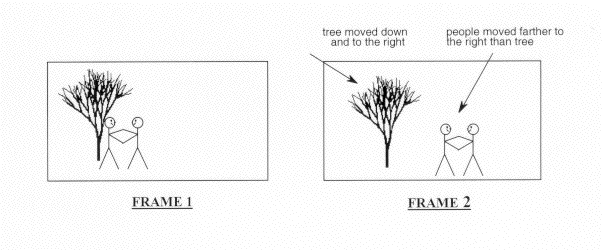
The temporal prediction technique used in MPEG video is based on motion estimation. The basic premise of motion estimation is that in most cases, consecutive video frames will be similar except for changes induced by objects moving within the frames. In the trivial case of zero motion between frames (and no other differences caused by noise, etc.), it is easy for the encoder to efficiently predict the current frame as a duplicate of the prediction frame. When this is done, the only information necessary to transmit to the decoder becomes the syntactic overhead necessary to reconstruct the picture from the original reference frame. When there is motion in the images, the situation is not as simple.Figure 7.17 shows an example of a frame with 2 stick figures and a tree. The second half of this figure is an example of a possible next frame, where panning has resulted in the tree moving down and to the right, and the figures have moved farther to the right because of their own movement outside of the panning. The problem for motion estimation to solve is how to adequately represent the changes, or differences, between these two video frames.
Final Motion Estimation Prediction Of course not every macroblock search will result in an acceptable match. If the encoder decides that no acceptable match exists (again, the "acceptable" criterion is not MPEG defined, and is up to the system designer) then it has the option of coding that particular macroblock as an intra macroblock, even though it may be in a P or B frame. In this manner, high quality video is maintained at a slight cost to coding efficiency.
Coding of Predicted Frames:Coding Residual Errors
After a predicted frame is subtracted from its reference and the residual error frame is generated, this information is spatially coded as in I frames, by coding 8x8 blocks with the DCT, DCT coefficient quantization, run-length/amplitude coding, and bitstream buffering with rate control feedback. This process is basically the same with some minor differences, the main ones being in the DCT coefficient quantization. The default quantization matrix for non-intra frames is a flat matrix with a constant value of 16 for each of the 64 locations. This is very different from that of the default intra quantization matrix which is tailored for more quantization in direct proportion to higher spatial frequency content. As in the intra case, the encoder may choose to override this default, and utilize another matrix of choice during the encoding process, and download it via the encoded bitstream to the decoder on a picture basis. Also, the non-intra quantization step function contains a dead-zone around zero that is not present in the intra version. This helps eliminate any lone DCT coefficient quantization values that might reduce the run-length amplitude efficiency. Finally, the motion vectors for the residual block information are calculated as differential values and are coded with a variable length code according to their statistical likelihood of occurrence.The MPEG Video Bitstream
The MPEG Video Bitstream is summarised as follows:- Public domain
tool mpeg_stat and mpeg_bits will analyze a bitstream.
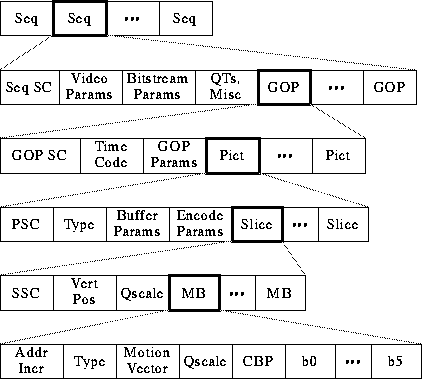
- Sequence Information
- 1.
- Video Params include width, height, aspect ratio of pixels, picture rate.
- 2.
- Bitstream Params are bit rate, buffer size, and constrained parameters flag (means bitstream can be decoded by most hardware)
- 3.
- Two types of QTs: one for intra-coded blocks (I-frames) and one for inter-coded blocks (P-frames).
- Group of Pictures (GOP) information
- 1.
- Time code: bit field with SMPTE time code (hours, minutes, seconds, frame).
- 2.
- GOP Params are bits describing structure of GOP. Is GOP closed? Does it have a dangling pointer broken?
- Picture Information
- 1.
- Type: I, P, or B-frame?
- 2.
- Buffer Params indicate how full decoder's buffer should be before starting decode.
- 3.
- Encode Params indicate whether half pixel motion vectors are used.
- Slice information
- 1.
- Vert Pos: what line does this slice start on?
- 2.
- QScale: How is the quantization table scaled in this slice?
- Macroblock information
- 1.
- Addr Incr: number of MBs to skip.
- 2.
- Type: Does this MB use a motion vector? What type?
- 3.
- QScale: How is the quantization table scaled in this MB?
- 4.
- Coded Block Pattern (CBP): bitmap indicating which blocks are coded.
Decoding MPEG Video in Software
- Software Decoder goals: portable, multiple display types
- Breakdown of time
       -------------------------
            Function      % Time
       Parsing Bitstream  17.4%
       IDCT               14.2%
       Reconstruction     31.5%
       Dithering          24.5%
       Misc. Arith.       9.9%
       Other              2.7%
       -------------------------
Intra Frame Encoding
Intra Frame Decoding
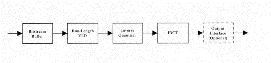
The input bitstream buffer consists of memory that operates in the inverse fashion of the buffer in the encoder. For fixed bit-rate applications, the constant rate bitstream is buffered in the memory and read out at a variable rate depending on the coding efficiency of the macroblocks and frames to be decoded. The VLD is probably the most computationally expensive portion of the decoder because it must operate on a bit-wise basis (VLD decoders need to look at every bit, because the boundaries between variable length codes are random and non-aligned) with table look-ups performed at speeds up to the input bit-rate. This is generally the only function in the receiver that is more complex to implement than its corresponding function within the encoder, because of the extensive high-speed bit-wise processingnecessary.
The inverse quantizer block multiplies the decoded coefficients by the corresponding values of the quantization matrix and the quantization scale factor. Clipping of the resulting coefficients is performed to the region �2048 to +2047, then an IDCT mismatch control is applied to prevent long term error propagation within the sequence.
The IDCT operation is given in Equation 2, and is seen to be similar to the DCT operation of Equation . As such, these two operations are very similar in implementation between encoder and decoder.
Non-Intra Frame Decoding
It was shown previously that the non-intra frame encoder built upon the basic building blocks of the intra frame encoder, with the addition of motion estimation and its associated support structures. This is also true of the non-intra frame decoder, as it contains the same core structure as the intra frame decoder with the addition of motion compensation support. Again, support for intra frame decoding is inherent in the structure, so I, P, and B frame decoding is possible.
This comment has been removed by the author.
ReplyDelete